Rank of the matrix Lecture 4
Topic: Linear system of equations with parameters
Summary
In the article I will show how to determine the number of solutions in linear system of equations with a parameter using the ranks of the matrix (and not Cramer’s rule, as usual).
Systems of linear equations with parameters
A linear system of equations with a parameter, for example:
 can be recognized by included cute letter
  , or:
, or:  . For different values of a (e.g.
 ) we will get different solutions of the system. Perhaps for some values we will get a system that has no solutions. Perhaps for some values we will get a system that has infinitely many solutions.
Our task is generally not to solve the system, but to determine for which parameter values the system has 1 solution (“unique solution”), infinitely many solutions (it is “undetermined”), and for which it has no solutions (“overdetermined”).
The number of system’s solutions depends on a rank of a matrix
To determine the number of solutions to the system, we can use Cramer’s rule and determinants, but in some systems it would be more convenient to use the Kronecker-Capelli theorem (or “Rouché–Capelli theorem”). Let’s recall what this theorem implys…
1. A system has 1 solution (“unique”) when:
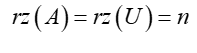 – the rank of the “coefficient matrix” A is equal to the rank of the “augmented matrix” U (which is A|B) and is equal to the number of system variables
2. A system is undetermined (has infinitely many solutions) when:
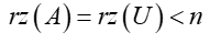 – the rank of the coefficient matrix is equal to the rank of the augmented matrix and is smaller than the number of system variables
3. The system is overdetermined (no solutions) when:
 – the rank of the coefficient matrix is different from the rank of the augmented matrix
General procedure
To use the rank of the matrix to determine the number of solutions to the equation depending on the parameter, we will proceed as follows:
– determined the rank of the coefficient matrix rz(A)
– determined for which parameter values the rank of the coefficient matrix rz(A) takes different values
– determined the rank of the augmented matrix
– determined for which parameter values the rank of the augmented matrix rz(U) takes different values
– determined the number of solutions to the system of equations depending on parameter values using conclusions from the Rouché–Capelli theorem
Before going further, you need to recall how to calculate the rank of the matrix!
Example
Let’s determine the number of solutions depending on the parameter ‘a’ in the system:
 First, we calculate the rank of the coefficient matrix A, i.e.:

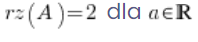
The rank of this matrix will be equal (after calculation which I pass here) 2. Please note that the rank of the coefficient matrix does not depend – in that specific case – on the parameter ‘a’ at all. The rank of matrix A would be always 2, no matter of ‘a’ parameter value. So at this time we do not write that for some ‘a’ the rank is equal to 1, for others 2, and for others 3. It is simply always equal to 2 for any given ‘a’. You can save:
Now we can calculate the rank of the augmented matrix U, i.e.:

This will be a bit more difficult, because the matrix whose rank we have to calculate contains the parameter ‘a’. However, we do not care about this – we treat ‘a’ as an ordinary number. Let’s “zero out” the third column, for example (we add the first row to the second one and multiply the first row by 4 and add it to the third one). We will get:

Notice that in the last column we do the most normal thing in the world: we multiply 1 by 4 and add it to ‘a’. Now we cross out the first rank and third column (according to the rules for calculating ranks) and increase the rank of the matrix by 1. We have:
![]()
Now we “zero” the second column by multiplying the first row by -3 and adding it to the second.
![]()
After deleting the third column, we get:
![]() Now let us note that the rank of the matrix that we have left after all these deletions depends on the parameter ‘a’.
Now let us note that the rank of the matrix that we have left after all these deletions depends on the parameter ‘a’.
If ‘a’ is equal to 5, the matrix will contain only zeros and the rank of the matrix will then be equal to 0. In this case, the rank of the augmented matrix will be equal to 2.
However, if ‘a’ is different from 5, the matrix will have a non-zero element and the row of the matrix will then be equal to 1. In this case, the row of the completed matrix will be equal to 3.
The above can be written:
 For
For 
 For different from
Summarizing the values of the ranks of the coefficient and augmented matrix, we get:
 For
For
 and For different from
That means, that the system has infinitely many solutions for (because then the rows of the matrix are equal and smaller than the number of unknown variables), and that there are no solutions for different from (because then the orders of the matrix are different).
The case where the system has 1 unique solution never occurs.
Click to remember how to solve systems of equations using matrix row (previous Lecture)< —
Click to see how to deal with systems of linear equations without using matrix row (next Lecture) –>