Econometrics Lecture 5
Topic: Pearson’s Linear Correlation Coefficient and Its Significance
The main goal of econometrics is to investigate and measure certain relationships occurring in economic phenomena. It simply explains the behavior of one variable depending on the behavior of other variables. It is therefore logical that the explanatory variables selected for the model  should be as strongly related as possible to the dependent variable
  . You are not going to explain, for example, annual fuel expenditures using the number of flights to the Moon. 🙂
So let us move on to how to name this relationship “properly” and how to measure its strength.
Statistical dependence, also known as CORRELATION, means a relationship between two random variables. Correlation analysis is used to “capture” whether such a relationship exists at all and to measure its strength.
What does a relationship mean? There is, of course, a similarity — at least by analogy — to human relationships. However, here it should be understood as a kind of similarity in the “behavior of two characteristics”. When one characteristic increases, does the other also increase? Or does it decrease? Or does it not change at all? For example, is there a relationship between crude oil prices and the stock price of a selected fuel company?
Intuitively, dependence between two variables means that knowing the value of one of them would allow us to predict the value of the other more accurately more often than without that information.
The most popular type of correlation is linear correlation. It concerns a linear relationship, i.e., if one thing increases, the other simultaneously either increases or decreases. Keep in mind, however, that quadratic, cubic, etc. relationships can also be analyzed.
Example 1
Is physical fitness related to the amount of milk consumed per week? To investigate this, 150 randomly selected people were asked about the average amount (in liters) of milk they consume per week, and their performance in a 500 m run was measured. So how can this relationship be measured?
To determine whether there is a relationship between the amount of milk consumed and physical fitness (understood here as the result in the 500 m run), a correlation analysis should be carried out. Ideally, it should be supported by specific mathematical calculations. This is where the correlation coefficient helps.
The most important measure of the strength of a linear relationship between two characteristics is Pearson’s linear correlation coefficient. It is calculated for measurable variables.
If variables are not quantitative but have, for example, an ordinal distribution, nonparametric correlation tests should be used. This is where ranking and Spearman’s rho correlation coefficient come in. In the case of nominal variables (gender, education, etc.), the strength of dependence is examined using Cramér’s V.
In this Lecture, however, I will focus on numerical values. Therefore, I will discuss only Pearson’s linear correlation coefficient, with particular emphasis on how to test its significance.
Pearson’s linear correlation coefficient
The general formula for calculating Pearson’s correlation coefficient for two variables X and Y.

Here you need to use the covariance between the variables divided by the product of their standard deviations. I showed all calculations step by step — including how to interpret the coefficient — in Lesson 2 (part 1) of my Course. I presented not only the “manual” computations, but also how you can do it quickly using Excel.
Typically, the result of a correlation analysis — the correlation coefficient — provides us with three pieces of information:
- Is the result statistically significant?
- What is the strength of the relationship?
- What is the direction of the relationship?
If the relationship is statistically significant, we can say that a relationship exists between the two characteristics (variables).
The correlation coefficient tells us about the strength of the relationship. It is expressed as a value in the range from -1 to 1. The farther the coefficient is from 0 (both positive and negative), the stronger the relationship.
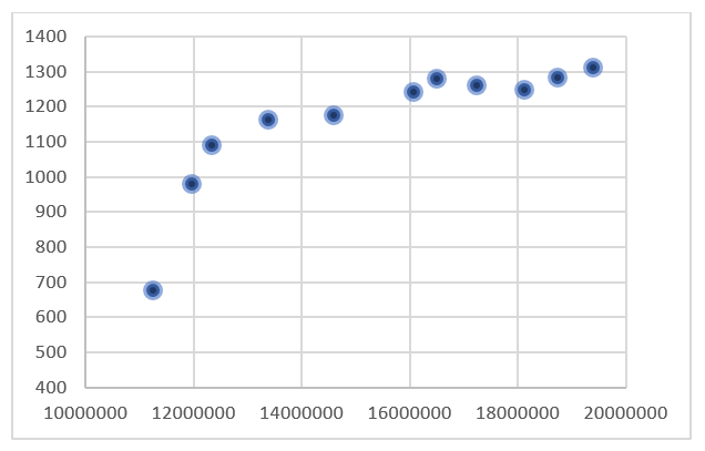
If the correlation coefficient is positive, we can say that when the values of one variable increase, the values of the other variable also increase (and conversely, when one decreases, the other decreases as well).
Example 2
If a significant, positive relationship were observed between weight and height in humans, one could conclude that taller people tend to have greater weight (taller people weigh more).
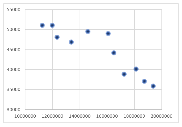
If the correlation coefficient is negative, we can say that when the values of one variable increase, the values of the other variable decrease (and conversely, when one decreases, the other increases).
Example 3
If a significant, negative correlation coefficient were observed between weight and height in humans, one could conclude that taller people tend to have lower weight (taller people weigh less).
A graphical interpretation of the correlation coefficient is the so-called scatter plot.
Examples of scatter plots for two characteristics X and Y:
or:
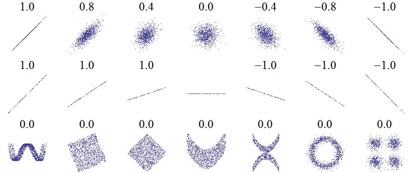
Below, look at a few examples of how the “cloud” of points is arranged depending on the value of Pearson’s linear correlation coefficient.
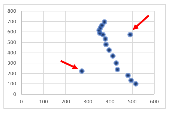
You should also be aware of certain pitfalls and limitations of this coefficient. Sometimes it may produce values that are not entirely reliable. This happens when the variable does not follow a normal distribution (which is the most preferred case). Another factor that may distort the correlation result is the presence of so-called outliers.
These points do not fully fit the rest of the data. A strong negative relationship can be observed here; however, the value of the correlation coefficient may be distorted by one or two outliers that skew the result.
Therefore, before moving on to calculations, first create a scatter plot for the two variables. If you notice any points that clearly deviate from the rest, remove that observation from the data set. However, this is a rather risky practice and is sometimes considered unacceptable.
Once you have created the plot and calculated the correlation coefficient, also test its significance.
Testing the significance of the correlation coefficient
The last issue I will discuss in this Lecture is the question of the significance of Pearson’s linear correlation coefficient. Does a similar relationship exist in the general population as the one observed in the sample? Or is it merely the result of chance? To examine this, we must assume that, at worst, both analyzed characteristics have distributions close to normal (a condition for using the test below). In the case of significant deviations from this assumption, nonparametric tests must be used.
The test of the significance of Pearson’s linear correlation coefficient is used to verify the hypothesis of no linear relationship between the studied characteristics in the population. It is based on Pearson’s linear correlation coefficient calculated for the sample. The closer the value of the coefficient r is to zero, the weaker the relationship between the studied characteristics.
The test statistic requires the null hypothesis  stated as follows: the true value of the correlation coefficient (from the general population, denoted as “rho”
  ) is equal to
  . This is equivalent to no correlation. The alternative hypothesis assumes that correlation exists between the variables, meaning that the coefficient is different from zero.

To verify this hypothesis, the following statistic is used:

where:
r — the value of Pearson’s correlation coefficient calculated from the sample,
n — the sample size.
Under the null hypothesis, the statistic t follows a Student’s t distribution with df = n-2 degrees of freedom.
From the t-distribution tables (included, of course, with the Course), or from a calculator, we read the critical value  for the previously assumed significance level
  . The significance level is a margin of error. It takes very small values, most often 0.05 or 0.01.
If the calculated value of t lies in the two-sided critical region  , then should be rejected in favor of the alternative hypothesis.
More precisely, when: — we reject . The correlation coefficient differs significantly from zero. Therefore, the variables are correlated.
 — there are no grounds to reject . The nonzero value of the correlation coefficient obtained from the sample occurred by chance.
Example 4
As an example, we will check whether the correlation coefficient between variables Y and X, equal to  , is significantly different from zero.
We set the null hypothesis  , against the alternative hypothesis
  .
.
I determine the test statistic for the null hypothesis, knowing that the number of observations in the sample is  :
:

For the significance level  and for
  degrees of freedom, I read from the Student’s t-distribution table the critical value
  .
.
Since , there are no grounds to reject the null hypothesis that variables Y and X are not significantly correlated.
On the basis of correlation, many more advanced analytical techniques have been developed, which makes it one of the most popular and widely used statistical measures.
This coefficient appears in econometrics in several places, primarily in methods for selecting variables for a model — in fact, in almost every method. Sometimes it happens that despite a high value of the correlation coefficient, it turns out to be insignificant. In that case, the relationship between the selected variables X and Y is not real. That is why, at the very beginning, before you choose a specific variable-selection method, you can eliminate some variables and save yourself further calculations.
END
Click to review where to obtain data and how to present collected data (previous Lecture) <–
Click to check what regression is and how the least squares method works (next Lecture) ->
Click to return to the Econometrics Lectures page