Assumptions of the Classic Method of Least Squares. And why classic?

No comments Join the discussion

Assumptions of the Classic Method of Least Squares. And why classic?

Joanna Grochowska

Learning Department Manager.

Graduated in Financial Mathematics and Computer Science and Econometrics from the University of Bialystok. Experienced tutor in mathematical and economic subjects. Associated with eTrapez since 2015.

She lives in Bialystok, Poland. She loves to travel and hike in the mountains. She enjoys meetings with friends, experiments in the kitchen and volleyball.

Econometrics Lecture 7

Topic: Classical Method of Least Squares – assumptions

This lecture will be devoted to the Classical Method of Least Squares. You can of course also come across the name Classical Linear Regression Model, KMRL for short. Both names are correct and both are safe to use.

I will present and briefly discuss all the basic assumptions of this method. They mainly concern certain properties of the random component.

It is worth knowing these assumptions, because very often this issue appears on the econometrics exam, but not only. I remember well that mentioning the assumptions of KMNK happened to me as one of the questions during the defense of my BA thesis 🙂

So I invite you to read!

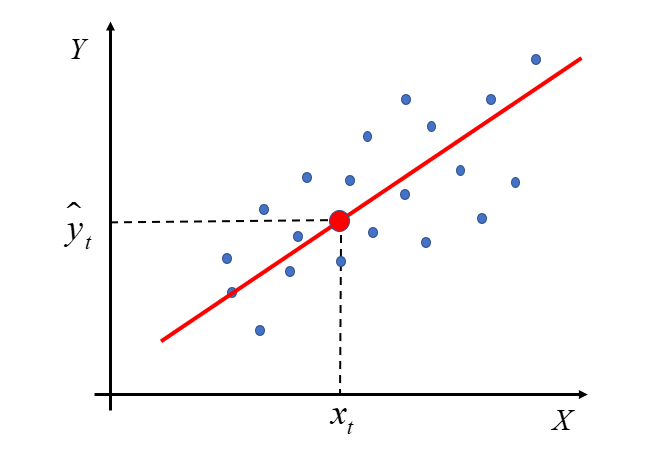
Let me start from the beginning, i.e. from the name itself. In the previous lecture the method of least squares was discussed. Its essence is best reflected in the example of a model with two variables – the explained one Y and one explanatory x The classic method of least squares is simply to determine under all conditions the applicability of OLS to estimate a vector $bold italic alpha$ in the model

$bold italic Y space equals space bold italic X bold italic alpha plus bold italic epsilon$

Here I will deal with the first part of the assumptions of the Classical Method of Least Squares. They are very important, because only when these assumptions are met, i.e. the actual data collected for the econometric model have the following properties interchangeably, only then can the model be built and the least squares method can be used to estimate the model parameters.

There are, of course, other methods of estimating model parameters, which have their own predetermined “guidelines”, e.g. the generalized method of least squares (UMNK), the method of maximum likelihood (MNW), the method of binomial regression, etc.

The assumptions of the KMNK are as follows:

The estimated econometric model is linear with respect to the parameters $alpha subscript j$ .
Explanatory variables $X subscript i$ are non-random quantities with fixed elements.
Matrix row $bold italic X$ is equal to the number of estimated parameters, i.e $r open parentheses bold italic X close parentheses equals k plus 1$ .
The sample size is larger than the number of estimated parameters, i.e. $n space greater or equal than space k plus 1$ .
There is no phenomenon of collinearity between explanatory variables.
The expected value of the random term is zero: $for all for t of space E open parentheses epsilon subscript t close parentheses equals 0$ .
The random component has a constant finite variance $for all for t of space D squared open parentheses epsilon subscript t close parentheses equals sigma squared$ ;
There is no phenomenon of autocorrelation of the random component, i.e. dependence of the random component in different time units $for all for t not equal to s of space cov open parentheses epsilon subscript t comma epsilon subscript s space close parentheses equals 0$ .
Random component has n -dimensional normal distribution: $epsilon subscript t space colon space N open parentheses 0 comma sigma squared close parentheses$ For t=1,2,…,n.

Note that there are a lot of them.

Perhaps you had less of them written down in your classes. For example, assumption $4$ and $5$ result from assumption no $3$ so they may have been omitted. Often, the last four random components are combined into one sub-clause.

I will now try to explain in more detail the meaning of each of the assumptions.

Assumption 1. The estimated econometric model is linear with respect to the parameters $alpha subscript j$ .

In one of the previous articles , I explained when an econometric model is linear with respect to parameters and when it is linear with respect to variables. Here, linearity with respect to unknown parameters is important $alpha subscript j$ .

In general, in a typically linear model, the sum of type products plays the main role . That is, both parameters and variables should be in prime powers at the same time, and the dependent variable Y should be a linear combination of explanatory variables and various parameters.

Hence, such a model can be written in matrix form: $bold italic Y space equals space bold italic X bold italic alpha plus bold italic epsilon$ .

Vector $epsilon$ is a vector of random components (individual observations) representing the combined effect of all secondary, random factors not included among the explanatory variables. Addition to the deterministic component of the random disturbance vector $epsilon$ is to model the fact that the recorded observations may differ in value from the values resulting from the theoretical construction of the economic model. Vector $epsilon$ groups random components that are by definition unobservable, we postulate their existence to explain any discrepancies between the theoretical values of the dependent variable and the observed values. In theory, if we know how many significant explanatory variables ( k ) there are and if we know what the form of the relationship is (linear), i.e. if Z1 is true, then the epsilon includes only random, secondary, disturbing factors. In practice, however, you have to take into account that the random component also includes the consequences of the following errors:

1. specification error (significant variable omitted, irrelevant variable included, etc.)
2. approximation error (if the form of the dependence is different, i.e., e.g. significantly non-linear, and it is not
approximated in a linear form).

In practice, we take into account that Z1 is not perfectly satisfied (but we can assume that we have chosen the explanatory variables well and that the true form of the relationship is well approximated by the linear relationship…). More precisely the property $epsilon$ will be described in points Z6-Z9.

Assumption 2. Explanatory variables $X subscript i$ are non-random quantities with fixed elements.

The explanatory variables are non-random. Their values are treated as constants in repeated trials.

The information contained in the sample is the only basis for estimating the structural parameters of the model.

Repealing this assumption results in the loss of essential properties of the estimators.

Assumption 3. Matrix row $bold italic X$ is equal to the number of estimated parameters, i.e $r open parentheses bold italic X close parentheses equals k plus 1$ .

The row of the matrix is the number of linearly independent columns. You can also say it’s the number of linearly independent rows. However, in the matrix notation, rows – reflect successive observations, while columns – successive explanatory variables $X subscript i$ . Therefore, it is about independence between the explanatory variables.

These assumptions ensure that the estimator can be determined uniquely.

Assumption 3 implies assumption 4 and assumption 5. Therefore, listing these assumptions separately is sometimes omitted.

Assumption 4. The sample size is larger than the number of estimated parameters, i.e. $n space greater or equal than space k plus 1$ .

The number of observations n should be greater than the number of estimated parameters (explanatory variables).

Assumption 5. There is no phenomenon of collinearity between explanatory variables

The explanatory variables cannot be collinear. observation vectors of explanatory variables (columns
matrix X) should be linearly independent.

The random component has its own specific properties that should be met under the assumption.

The formation of the random component in econometric model in its general form is one of the basic sources of knowledge about whether the model has been built correctly.

Its value is the difference between the empirical value in a given period $y subscript t$ and the estimated theoretical value for the values of explanatory variables in a given period.

By definition a model (in a broad sense) is a simplified picture of reality. In this case, when building an econometric model, we want to “simplify” certain phenomena occurring in economics, to the form of a function. At the same time, we expect that the model will reflect reality as best as possible, thus the difference between the value that occurred in reality (empirical) and what we calculated on the basis of the model (theoretical) will be as small as possible, i.e. as close to zero as possible.

The properties of the random component are listed below. Although they sound complicated, it is easier than it sounds.

Let’s start with the fact that if the random component was shaped according to some pattern, then we could hardly talk about any randomness. For us, this would only mean that “something is going on” in this rest, and the model was not built correctly. If we see that something is going on, we should find out what is hidden there. Most likely, in the values of the random component, in the case of its autocorrelation, there is a factor that has a significant impact on the formation of the dependent variable. A factor that we did not take into account when considering what may affect the issue we are investigating. One of the quick methods aimed at the expected decrease in the autocorrelation coefficient is to add an endogenous variable lagged in time to the model, but more on that later because it is a much more complicated matter.

Assumption 6. The expected value of the random term is zero: $for all for t of space E open parentheses epsilon subscript t close parentheses equals 0$ .

The expected values of the random components are equal to zero ( $for all for t of space E open parentheses epsilon subscript t close parentheses equals 0$ for t=1,2,…,n). This means that the disturbances represented by the random components tend to reduce each other.

Assumption 7. The random component has a constant finite variance $for all for t of space D squared open parentheses epsilon subscript t close parentheses equals sigma squared$ .

Random component variances $epsilon subscript t$ are constant, i.e. $for all for t of space D squared open parentheses epsilon subscript t close parentheses equals sigma squared$ for t=1,2,…,n. This is the so-called homoscedasticity property.

The matrix of variance and covariance between residual terms is of the form

$D squared open parentheses epsilon close parentheses equals E open parentheses bold italic epsilon bold italic epsilon to the power of T close parentheses equals sigma squared bold italic I equals open square brackets table row cell sigma squared end cell 0 midline horizontal ellipsis 0 row 0 cell sigma squared end cell midline horizontal ellipsis 0 row vertical ellipsis vertical ellipsis down right diagonal ellipsis vertical ellipsis row 0 0 midline horizontal ellipsis cell sigma squared end cell end table close square brackets$

This assumption ensures that the value of the disturbance variance does not depend on the number of observations.

Assumptions 6 and 7 determine the favorable properties of the estimator $bold italic a$ parameter vector $bold italic alpha$ but more on that in the next lecture.

Assumption 8. There is no phenomenon of autocorrelation of the random component, i.e. dependence of the random component in different time units $for all for t not equal to s of space cov open parentheses epsilon subscript t comma epsilon subscript s space close parentheses equals 0$ .

Random components $epsilon subscript t$ and $epsilon subscript s$ they are independent of each other. There is no so-called autocorrelation of random components.

This means a linear relationship between model residuals that are “k” periods apart. This applies to dynamic models.

Its occurrence means that one of the significant explanatory variables has been omitted in the model or an incorrect form of the model has been adopted .

Assumption 9. Random component has n -dimensional normal distribution: $epsilon subscript t space colon space N open parentheses 0 comma sigma squared close parentheses$ For t=1,2,…,n.

Each of the random ingredients has $epsilon subscript t$ has a normal distribution.

This assumption concerning the normality of the distribution of the random component is important in statistical inference.

If all the above four assumptions in the case of the model we are analyzing turn out to be true, then we can understand the disturbing components as generated by the white noise process . In this case, all autocorrelation coefficients and partial autocorrelation coefficients will be zero, statistically insignificant. To determine if there is white noise, we need to test the relevant hypotheses. These include, for example, Quenouille statistics or Durbin-Watson statistics.

In the above Lecture I tried to bring you closer to the assumptions of the Classical Method of Least squares.

This lecture should actually be preceded by a lecture on the Method of Least Squares, because first the assumptions should be made, then the application of the method and deriving formulas for parameter estimators $alpha subscript j$ model.

I hope that since you already know what the Least Squares Method is and you have learned the assumptions of the applicability of this method, then linear regression will be closer to you and not so scary 🙂

END

Click to revisit what regression and Least Squares are all about and where the formulas for estimating structural parameters come from (previous Lecture)< –

Click here to return to the Econometrics Lectures page

Are you looking for college or high school math tutoring? Or maybe you need a course that will prepare you for the final exam?

We are "eTrapez" team. We teach mathematics in a clear, simple and very precise way - we will reach even the most knowledge-resistant students.

We have created video courses translated in an easy, understandable language, which can be downloaded to your computer, tablet or phone. You turn on the video, watch and listen, just like during private lessons. At any time of the day or night.