In this article, I will introduce a method for solving systems of linear equations, called the „inverse matrix method”. It can be safely added to the known methods: Cramer, Kronecker-Capelli (this is a proper transition to the Cramer method) and Gauss.
We make a reservation right away that the inverse matrix method can only be used in systems of linear Cramer equations, i.e. those in which:
- There are as many equations as there are unknowns
- The main determinant of the system (composed of coefficients with variables) is different from zero
1. General case
What is the method? Let’s take a system of equations that satisfies the above assumptions:

The system has as many equations as it has unknowns (n equations and n unknowns), and its principal determinant is different from zero:

The above system of equations can be written as a multiplication of the following matrices:

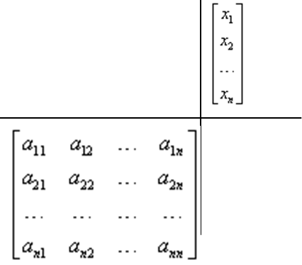
You do not believe? Check for yourself by multiplying the matrices in the appropriate table
 and
and![]() :
:

Multiplying the first row by the first (and, of course, only) column, we get:
a_{11} x_{1} +a_{12} x_{2} +...+a_{1n} x_{n} – so exactly the left side of the first equation, which should be equal to b_{1} . This will be the same in the following lines, and you can see that our system of equations and the matrix equation are equivalent. So we go back to the matrix equation:

To solve it, we multiply both sides by (inverse matrix) – as it was usually done in matrix equations:

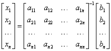
Note that we multiply both sides, but from the left side, because the coefficient matrix is on the left side of the matrix of unknowns. The inverse matrix will exist because its determinant is different from zero, which we ensured in the assumptions (this is the Cramer system). So we go to:

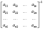
Now all we have to do is compute the inverse matrix: ,
,
multiply it by the matrix: ![]()
…and we get the resulting matrix:
![]() and from there you just need to save the answer 🙂
and from there you just need to save the answer 🙂
2. Example
Let’s take a specific system of linear equations:

At the beginning we write the matrix form of this system: 
Notice that in the first matrix from the left there are the coefficients for the variables of the system, then there is the matrix of unknowns (one-column), and on the right there is the matrix of intercepts. Now it is enough to solve this equation as you solve matrix equations, i.e.:

Then compute the inverse matrix: 
we should get: 
and multiply it by: 
…we should then output:

Now all that’s left to do is save the answer:
answer .
.
3. Summary
The inverse matrix method has the advantage that you don’t need much new knowledge to learn it other than the ability to calculate inverses and solve matrix equations.
Its disadvantage, however, is the great tediousness of calculations and the limitation to Cramer systems.
Systems of equations that have more than three equations and unknowns require the calculation of inverse matrices larger than 3 \times 3 dimension. This requires the use of a method other than counting from the complement matrix. It is:
Gauss-Jordan Inverse Matrix (next Lecture) –>
Click to recall how to solve systems of linear equations with a parameter (previous Lecture)< —
