Econometrics – Lecture 6
Topic: Regression analysis. Estimation of model parameters
using the Least Squares Method.
In this lecture, I will explain what linear regression is and how the Least Squares Method works in detail. You will therefore learn where the formulas for estimating the structural parameters  of an econometric model come from.
Welcome!
The main goal of econometrics is to examine and explain the behavior of one economic variable as a function of the behavior of other variables. Of course, these variables must be related in some way. For example: whether and how a household’s expenditures depend on its income; or whether the increase in food expenditures is faster or slower depending on income growth.
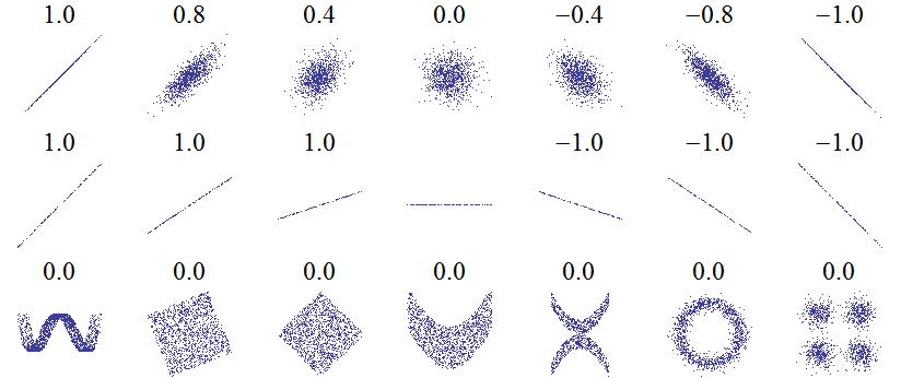
In one of the previous lectures, I discussed a type of statistical dependence known as correlation. As we remember, the concept of correlation concerns the STRENGTH and DIRECTION of the relationship under study.
Besides correlation analysis, there is another type of analysis that can be performed—namely REGRESSION. It is a branch of statistics concerned with studying relationships and dependencies between the distributions of two or more examined characteristics in the general population.
However, the term regression refers to the SHAPE of the relationship between characteristics. We distinguish between linear and nonlinear regression analysis.
The graph of linear regression for two variables, as the name suggests, is a straight line. In nonlinear regression analysis, the graphical representation of the relationship consists of higher-order curves, e.g., a parabola.
It is enough to look at the point clouds below. Based on them, one can conclude that the closer the values of the correlation coefficient are to  (in absolute value), the more linearly the points are arranged on the chart. The third row shows examples of nonlinear plots.
Source: https://pl.wikipedia.org/wiki/Zależność_zmiennych_losowych, accessed on 12 June 2018.
Regression and correlation analysis may concern not only two, but also a larger number of variables. In such cases, we speak of so-called multiple analysis.
I will now proceed to discuss both the simple and the multiple case of linear regression.
Linear regression – introductory information
The term linear regression comes from the fact that the assumed model of dependence between dependent and independent variables is a linear function or a linear transformation.
The line determined by the equation of a linear model is the regression line, and the model itself is a linear regression model. One can speak of a regression line only in the case of a model with a constant term and one explanatory variable. In the multidimensional case, i.e., multiple regression, we speak of a regression hyperplane.
Before more detailed charts appear, it is worth recalling the general form of an econometric model:

Taking into account realizations of the variables, it is often written as follows:

where:
 – the explained (dependent, endogenous) variable; realizations of the dependent variable in period t,
 – explanatory (independent) variables; realizations of the explanatory variables in period t,
 – the random (error) term (you can read more about it in the article),
 – successive realizations (observations),
  .
.
The origin of the term regression is quite interesting.
In everyday language, regression means: going backward, decline, disappearance. So you might wonder—how did this word end up in statistics?
The term was first used by Francis Galton, Charles Darwin’s son-in-law. In 1886, he studied the relationship between the height of parents and the height of their children. He observed that tall parents tend to have, on average, tall children. However, the children of exceptionally tall parents tend to be closer to the average height than their parents are. Galton called this tendency to return toward the mean “regression toward mediocrity.” His conclusions can therefore be expressed using the following linear model:

where the value of the parameter standing next to the explanatory variable lies between  . This means that one centimeter of the parents’ height translates into less than one centimeter of the children’s height.
The dependent variable and the explanatory variables in a regression model are not symmetric. In his research, Galton not only assumed that parents’ height affects children’s height, but also that the effect does not work in the opposite direction—i.e., parents’ height does not depend on children’s height.
Therefore, it is worth noting that in economic theory it is very important to know the direction of the cause-and-effect relationship.
Simple linear regression
Simple linear regression concerns the case of two variables: the dependent variable Y and one explanatory variable X.
A straight line can be described using a formula you have known for years (since middle school):  . This is the simplest notation. So if we already know what the letters Y and X mean, then the remaining two represent:
– the parameter associated with the explanatory variable; this is the slope coefficient of the regression, i.e., the tangent of the angle  between the line and the OX axis,
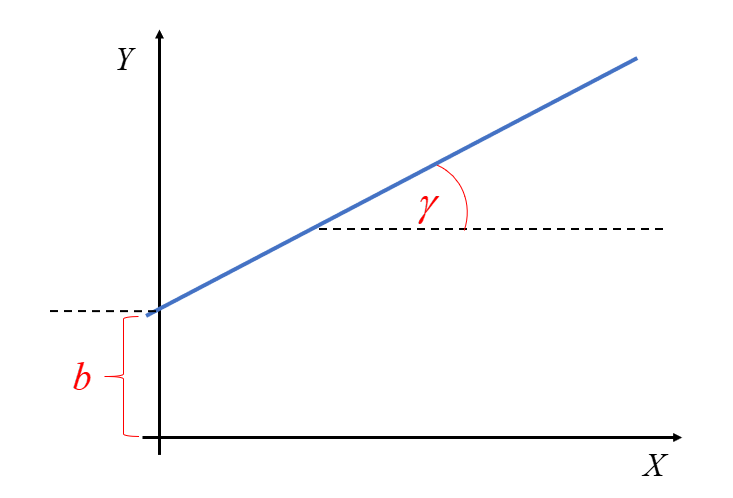
 – the intercept (constant term), i.e., the coordinate of the point where the line intersects the OY axis.
Most people probably remember how, in high school (or earlier), you found the equation of a line passing through two points  and
and  . Of course, there was a specific formula for this, available for example in exam formula sheets:
  . Equally well, it was enough to solve a system of two linear equations by substituting the coordinates of the points for X and Y, for example:
  and from that compute the unknown parameter values and .
It is worth remembering that in econometrics, however, we do NOT deal with a functional relationship (often called deterministic), i.e., one in which each value  corresponds to one and only one value
  .
.
In econometrics, we study stochastic (random, probabilistic) relationships between the variables X and Y. In this case, EACH value corresponds to an entire set of values forming a certain distribution. Hence, the typical equation of a simple regression line is as follows:

This situation can be illustrated as follows:
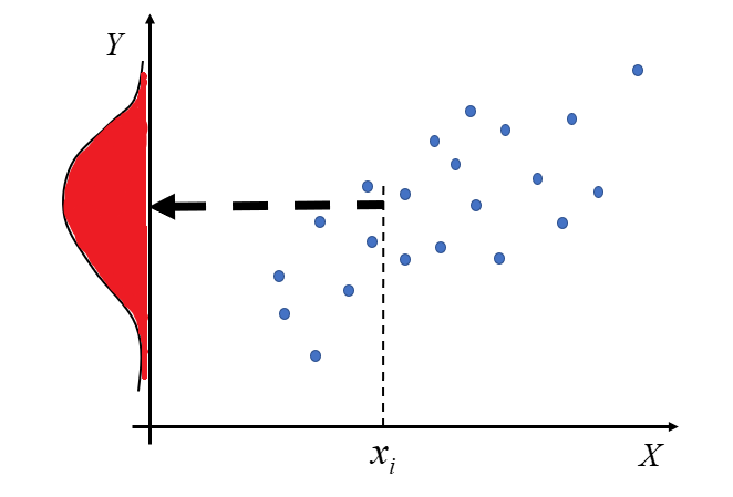
If this distribution is a normal distribution (one of the types of statistical distributions of random variables), then the relationship Y(X) is linear.
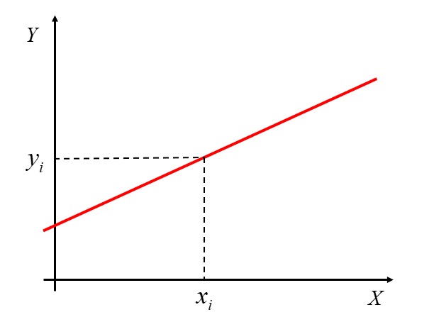
Let’s get to the point. Drawing a straight line through two points seems easy enough. However, with many points it won’t be that simple. In practice, it is almost never the case that one line passes through every point marked on the chart.
In such a situation, we need to choose a method that allows us to find the most optimal line. It should be properly “fitted,” i.e., drawn in a way that best reflects the relationship between X and Y.
Such a line (that is, the regression equation in its THEORETICAL form) is written as:

If we take into account specific realizations of the variables in subsequent periods t, we can also write it as:

In this case,  is an estimator, i.e., the estimated value of the intercept. Meanwhile,
  represents the estimated value of the regression coefficient. It determines the influence of variable X on variable Y.
The question is: how do we express numerically the values of the parameters and ? Should I draw a line, for example,  , or rather a line with a slightly different slope, for example
  ?
?
In the next part of the lecture, I will explain mathematically how to derive the formulas for the best estimates of and , as well as the remaining parameters  for the case of a model with many explanatory variables.
Estimation of the parameters of an econometric model using the Least Squares Method – the case with one explanatory variable.
There are many methods for estimating model parameters. Perhaps you have already heard of maximum likelihood, median regression, or the two-point method. Nevertheless, among all these methods the most popular one is the Least Squares Method (often abbreviated as LS).
It requires certain assumptions, which I will discuss in more detail in the next lecture. The most important of them concern the properties of the random error term  in the model
  :
:
- the expected value of the error term equals zero
 ;
; - the error term has a constant finite variance ;
- there is no autocorrelation of the error term, i.e., no dependence of the error term across different time periods .
 ;
; ;
; .
.For the sake of consistent notation, in the article above and throughout my entire course I use the following symbols: and . These are least-squares estimators of the parameters  and
and  from the model:

In your classes, you may have used a more general notation, such as:
So you were looking for parameter estimates in the theoretical form:
 .
.
In the literature or during classes you may also encounter the reversed notation:
 , so the theoretical equation of the line would be:
 .
.
The most important thing, however, is to understand which letter in the equation denotes the intercept and which denotes the slope coefficient (the one multiplying X).
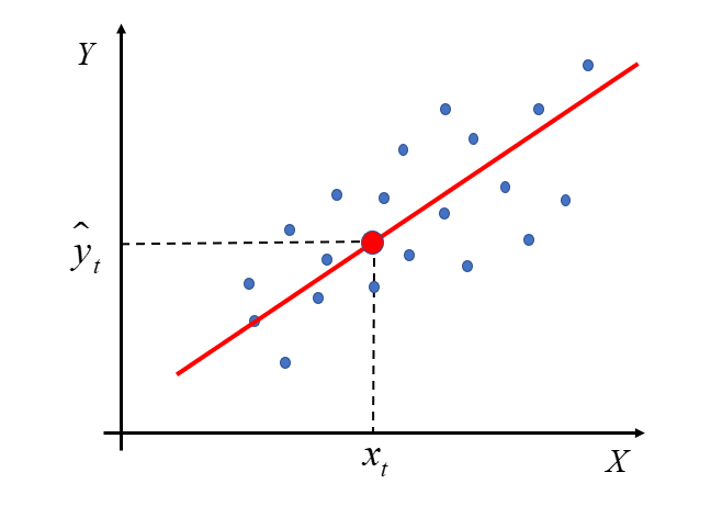
At this point, go back for a moment to the chart shown earlier. As I mentioned, the red line does not perfectly match all the blue points. Some of them lie below the line, others above it.
The econometric model will be better fitted the smaller the distance between the theoretical values  and the observed values
  .
.
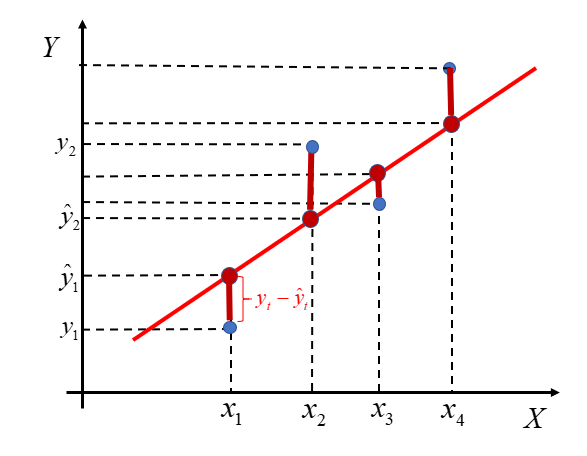
Each of these vertical (burgundy) segments represents the difference between the actual values of the variable and the theoretical values computed from the regression line. These are the model’s so-called residuals. We denote them by:

The relationship between residuals, observations, and estimated parameters can be written as:

This implies that the residuals  are estimates of the random terms from the model
  , but they are not equal to them!
Some differences between actual and theoretical values lie above the axis, so they are positive. Others lie below the axis, so they are negative. Therefore, if our goal is to make these segments as small as possible, it makes no sense to simply add the raw differences  . In that case, the result would not be meaningful. The fit is better the smaller the absolute values of these deviations are.
Example 1
In a certain model, the differences between the theoretical and the actual values are: . These are distances between two points. You can compare them, for example, to a temperature reading on a thermometer and its distance from zero—sometimes it is positive, sometimes negative. Or to steps taken forward (the positive ones) and backward (the negative ones).
If you need to compute the overall difference, i.e. add up all distances, a simple sum of the numbers will not be meaningful: . Many numbers simply cancel out. But you did not take only four steps backward. That is why you should use the absolute value of each number, i.e. its distance from zero on the number line. It’s like counting steps—forward and backward—together.

Now everything matches 🙂
The criterion that must be minimized in order to obtain the best fit is the sum of the absolute values of all residuals:

To find the smallest values—i.e. the local extrema of a multivariable function—we need derivatives (you can find more about them in Krystian’s courses).
However, this function is inconvenient to work with, because the absolute value function has no derivative at zero. As a result, the sum  cannot be minimized using standard analytical methods.
The Least Squares Method comes to the rescue. As the name suggests, it allows us to search for a minimum of the sum of squared differences between observed values and theoretical values (computed from the model equation):

Substituting the theoretical model equation, we obtain:

We now need to find the minimum of the sum-of-squares function  . That is, we choose the estimates
  , so that this sum is as small as possible.
Using calculus, we can find an extremum of a function. Here it is enough to compute the partial derivatives with respect to the parameters and set them equal to zero. For the function these conditions can be written as a system of equations:

To compute the partial derivatives, we can of course expand the squared expression in parentheses, i.e.:

By computing the partial derivatives and using the basic derivative rules, namely:  ,
,  ,
,  , and
, and  , I obtain:


Comparing the computed derivatives to zero, I get:


0«/mo»«munderover»«mo»§#8721;«/mo»«mrow»«mi mathvariant=¨normal¨»t«/mi»«mo»=«/mo»«mn”>1«mi mathvariant=¨normal¨»n«msub>«mo»+«/mo»«msub>a1«munderover>∑=1«mo> «msubsup>x2«mo>=«mn>0«mspace linebreak=¨newline¨/»«/math»” />

Our task is to solve the above system of equations and compute the values of and .
I will use here the method of opposite coefficients.


0«munderover>∑=1«msub>«mo>+«msub>a1«munderover>∑=1«mo> «msubsup>x2«mo>=«munderover>∑=1«msub>«msub>«mo>/«mo>·«mi mathvariant=¨normal¨»n«mspace linebreak=¨newline¨/»«/math»” /> 0«munderover>∑=1«msub>«mo>-«msub>1«msup>∑=1«msub>2«mo>=«mo>-«munderover>∑=1«msub>«munderover>∑=1«msub>«mtr>«mi mathvariant=¨normal¨»n«mo> «msub>0«munderover>∑=1«msub>«mo>+«mi>n«mo> «msub>a1«munderover>∑=1«msubsup>x2«mo>=«mi>n«munderover>∑=1«msub>«msub>«mspace linebreak=¨newline¨/»«/math»” />
Adding both equations together, we get:

1«munderover>∑=1«msubsup>x2«mo>-«msub>1«msup>∑=1«msub>2«mo>=«mi>n«munderover>∑=1«msub>«msub>«mo>-«munderover>∑=1«msub>«munderover>∑=1«msub>«mspace linebreak=¨newline¨/»«/math»” />
Hence we can compute the value of the estimator 1«/math»” />:


After a few small transformations, we finally get (for readability I won’t write the summation indices):
It remains to estimate the parameter . For this purpose, I will use the first equation from system (1).


Hence, finally:
where  and
and  are the arithmetic means of the variables X and Y, respectively.
After some transformations, one can also use another form of the formula for the parameter in front of X. Both forms are correct and can be used interchangeably.
This is how we derive the formulas for estimating the structural parameters of an econometric model. 🙂
For those who are more mathematically advanced: how do we know that the values computed in this way actually minimize the function ? In mathematical analysis, to confirm this one typically starts by computing the second-order partial derivatives of the function with respect to the parameters. I remember that the first derivatives looked as follows:  and
and  .
.


I arrange them into the so-called Hessian, i.e. the matrix of second-order derivatives:

A function of two variables has an extremum when two conditions hold:
- a local maximum when the determinant of the matrix at the point is positive, i.e. and
- a local minimum when the determinant of the matrix at the point is positive, i.e. and
 is positive, i.e.
  and
and 

I am looking for the value that minimizes the function .
The second condition for a local minimum is satisfied because  . Therefore, I check the determinant of the Hessian to make sure it is indeed positive. For a
  matrix, the determinant is easy to compute:
  . Hence:


Therefore, the derived estimators of the parameters and minimize the function .
Interpretation of the slope coefficient and the intercept
Once you compute the parameters of the linear regression equation , it is worth knowing what they actually mean.
We interpret the estimated value of the slope coefficient as follows:
An increase (ALWAYS an increase) of the explanatory variable X by 1 unit implies a change (an increase or a decrease) in the explained variable, on average, by the value of the estimated parameter
The intercept tells us what value of Y we should expect when X equals zero. However, this interpretation is not always meaningful. I mentioned this in my course.
Example 2
In a certain group of students, the relationship between the number of points obtained as an exam score , and the number of hours spent studying for that exam was examined. After calculations, the following model was estimated: . The interpretation of the model parameters is as follows:
– if the number of hours spent studying for the exam increases by one hour, then the number of points obtained on the exam increases on average by about 37 points;
– is not interpretable. After all, it makes no sense to say that if a student does not study for the exam (spends hours studying), they will obtain as many as 128 points on the exam…
Estimation of econometric model parameters by the Least Squares Method – the case of multiple explanatory variables.
A moment ago, I explained how searching for a line works in the case of two variables X and Y. A linear model with an intercept and one explanatory variable is a special case of a model with k explanatory variables. So how does the Least Squares Method work when we have more than one X variable? In this case, finding a solution becomes relatively straightforward when we use matrix algebra.
The general econometric model with an intercept has the form:
In matrix–vector notation, it can be written as:

Hence:

With this notation, the column vector contains all observations of the dependent (explained) variable. In the matrix  , successive columns contain observations of the explanatory variables in the model. Typically, the matrix is a rectangular matrix with many more rows than columns, because most often the number of observations is greater than the number of variables
  . A rectangular matrix cannot be inverted (only square matrices are invertible). For this reason, equation (2) cannot be solved using purely algebraic manipulations.
After estimating the structural parameters  , the econometric model will take the form:

Now I will show how to derive the estimator  of the parameters using the Least Squares Method.
The principle is the same as before. The idea of OLS comes down to choosing the estimated values  of the structural parameters
  , so that the sum of squared differences between the observed values and the theoretical values computed from the model equation is as small as possible.
As before, after substituting the theoretical model equation, I obtain:

The solution of the system in matrix form will be a vector of the form:  .
.
The function  , using the properties of matrix operations, can be written in matrix form as follows:

The sum of squared residuals  is a single specific number — in other words, a scalar. Therefore, each term in the obtained sum is also just an ordinary number. Transposing scalars or changing the order of multiplication does not affect the result, so:
  . As a result, we get:

The function attains a minimum if its first derivative with respect to the vector equals the zero vector, and the second derivative is positive definite.

Setting the derivative  equal to the zero vector, I obtain:


Using the property of matrix multiplication for a matrix  and its inverse
  , we obtain the identity matrix, i.e.
  . This is the matrix corresponding simply to the number one.
Hence, we finally obtain the formula for the estimates of the unknown structural parameters in vector form:

 denotes the transpose of the matrix , while
  denotes the inverse of the matrix
  .
.
So far, we have considered the necessary condition for the existence of an extremum. We must now verify whether the extremum we found is indeed a minimum of the function . The sufficient condition for an extremum is that the Hessian matrix (the matrix of second derivatives) is positive definite. In this case, it takes the form:

The equation above clearly shows that the positive definiteness condition for the Hessian is satisfied, because is positive definite as long as its determinant is non-zero.
Interpretation of the coefficients
As in the case of an equation with a single explanatory variable, it is also useful to know how to interpret the parameters of the linear regression equation .
In this case, our line of thinking should follow the previously discussed single-variable case very closely. The difference is that we must add the phrase indicating that the remaining variables (not being interpreted at a given moment) are held constant. Consequently, the estimated value of the coefficient  , associated with the variable
  , where
  , is interpreted as follows:
An increase (ALWAYS an increase) in the explanatory variable
 on average by the value of the estimated parameter
 As before, the intercept tells us what value of Y we should expect when all explanatory variables are equal to zero. However, for economic variables this interpretation is not always meaningful, as shown in Example 2.
This is where the formulas for estimating the parameters of the econometric model using the Least Squares Method come from, and this is how they were derived.
Fun fact – Anscombe’s quartet
Everything that has upsides also has its downsides. One example illustrating the limitations of the Least Squares Method in the general case is Anscombe’s quartet – a specially constructed set of four datasets that have nearly identical statistical indicators (the mean and variance in the X and Y directions, the correlation coefficient, and the regression line), despite having a markedly different structure when viewed graphically.
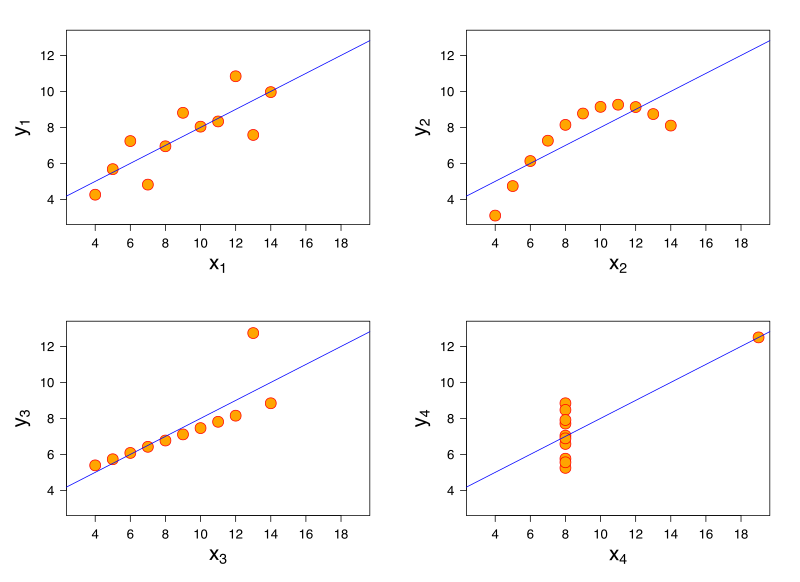
Source: By Anscombe.svg: SchutzPrace; derivatives of this file (label using subscripts): Avenue – Anscombe.svg, CC BY-SA 3.0, https://commons.wikimedia.org/w/index.php?curid=9838454, accessed: 15 June 2018.
At the very end of this article, I will mention one more important property. Using the Least Squares Method, the resulting estimators of the model parameters have the following properties: they are linear, consistent, unbiased, and most efficient. But more on all of that in the next lectures.
Summary
In the lecture above, I presented the concept of “regression” and the operation of the most widely used estimation method in econometrics, known as the Least Squares Method. It is precisely with this method that, by estimating the unknown parameters of the model, we obtain estimates for which the model best fits the presented data.
I hope that from now on the formulas used will no longer be a mystery to you.
If you want to apply this knowledge in practice, I encourage you to take a look at my course, especially lesson no. 3.
THE END
Click to see what the assumptions of the classical least squares method are (next lecture) ->
Click to return to the page with Econometrics lectures