Quick Regression in Excel – The Little-Known REGLINP Formula

---

One of the super important steps in the econometric modeling process is estimating its parameters. In my Econometrics Course, I dedicated the whole Lesson 3 to this topic.

In the lesson, I showed how to manually calculate the structural coefficients of the model. This was done using direct formulas (you know, the ones with sums) in simple regression, and the matrix method in multiple regression. All of this, of course, was using the Least Squares Method.

However, very often in classes or when working on various econometric projects, MS Excel is used for calculations. There, with the “REGRESSION” function, you can quickly and easily get almost all the necessary results for estimation and later verification of the model. That’s also something I covered in my Course.

In this article, I’d like to show you another additional function used in Excel. It’s the REGLINP() formula.

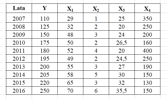
I have such an example econometric model, describing the relationship of a house’s value based on four explanatory variables:

– value of the house [in thousands of PLN]

– square footage [in ]

– floor number

– annual income of the buyer [in thousands of PLN]

– distance from a service center/store, etc. [in m]

Here are the precise details:

So, I’m going to estimate the model parameters:

.

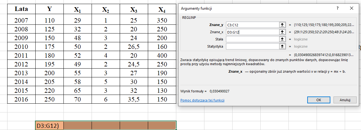
I’m going to use the REGLINP() function for this.

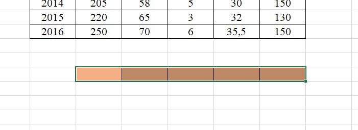
This function is an array function. So, before you select it, I mean, before you insert the REGLINP() function, you’ve got to prepare a space for the result, meaning select as many cells in the ROW as there are model parameters. In our case, that would be 5 cells (from to ).

Now select from the menu under FORMULAS –> INSERT FUNCTION. Then, in the pop-up that appears, look for the REGLINP function.

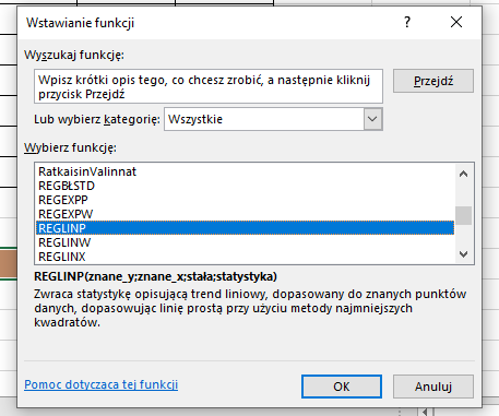
After hitting OK, a window like this should pop up for you to fill out:

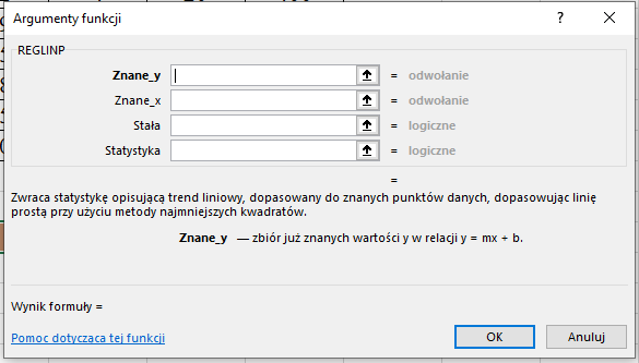
Alright, let’s fill this out.

“Known_y” is the range of numerical values for the dependent variable Y. Meanwhile, “Known_x” is the range for all the explanatory variables . Just place your cursor in the cell in the window and then select the range of all relevant numbers from the data table.

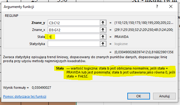
Next up, we fill in the last two formulas. First up, “constant”. You’ve gotta enter one of two values here – 0 or 1. It depends on whether our model includes a constant, meaning if it has an intercept or not. In our case, there’s an intercept, so I’m putting “1”.

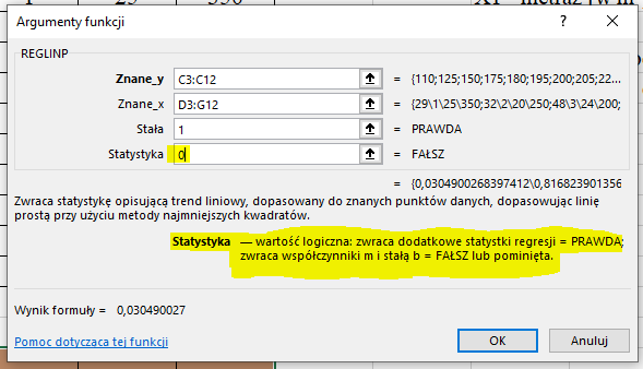
The last cell to fill: “statistics”. Just like above, you can enter two logical values: 0 (false) – if you just want the coefficient values for estimation, or 1 (true) – if you want additional statistical values of the econometric model to be displayed (like standard errors, the coefficient of determination, etc.)

Now it would be a good time to click OK and wait for the result to show up.

But wait a sec! After clicking “OK”, indeed, the result will show up, but only in the first cell… What about the rest?

Remember, with array formulas in Excel, to get the final result in all cells, you can’t just click OK; you need to use the keyboard shortcut:

<CTRL>+<SHIFT>+<ENTER>.

Only then will our final and correct result appear:

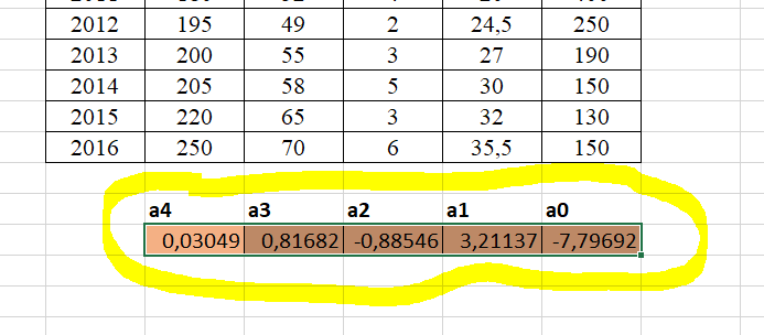
And another crucial tip – the estimated parameter values are read BACKWARDS. Yeah, someone programmed it that way 🙂

So, our estimated model looks something like this:

.

Hope you dig this extra option in Excel. Of course, I invite you to my course, where you’ll find out what to do next with such an estimated model 🙂