
Econometrics Lecture 3
Topic: Random Component
At the end of the previous Lecture 2, I mentioned one of the reasons why the random component is important in an econometric model. Thanks to its presence, the model takes on a stochastic rather than a deterministic character.
I assume that this last sentence may not be entirely clear. In this Lecture, I will explain what it means.
Let us first focus on the definitions of the terms deterministic and stochastic. According to the Polish Dictionary:
- Deterministic means “causally conditioned”, “non-random”; all phenomena and actions are connected by cause-and-effect relationships and are therefore unambiguous.
In this sense, using the term deterministic simply means dealing with something precisely specified.
- Stochastic (from the Greek stochasis – conjecture) means “random” or “chance-based”.
Here, therefore, we are dealing with something more abstract — not determined with 100% precision.
In mathematical notation, you may encounter the following types of models:
DETERMINISTIC MODELS – models that do not include a random component, that is  . This is an ordinary, concrete function, for example a linear one
  . In a more econometric notation, this model takes the following form:
  . This means that each value of the explanatory variable
  corresponds to a specific value of the variable
  .
.
STOCHASTIC MODELS – models that include a random component, that is  . In the case of a linear function, the model would take the form
  . In this case, however, values of are not assigned unambiguously to values of the variables .
The question then arises — why do most econometric models take this second form? Let us consider a few real-life situations.
Example 1
Ms. Magda receives a monthly allowance. It is a fixed, regular amount that she can spend on any additional purchase. Most often, she buys some nice clothes at a bargain price. However, from time to time she decides to stock up on cosmetics or buy other necessary items.
Ms. Magda’s purchasing decisions are determined primarily by prices — more precisely, promotions — as well as by her own free choice.
Example 2
You decide to plan meals for your family (four people) for the next month. Standing in front of the menu choice, would you eat the same meal every day? You naturally take prices and availability into account.
You go shopping. After making your choices, you happily head toward the checkout, but on the way you notice other, cheaper products. You decide they are a better deal. You change everything, and with the money saved you buy something extra for dessert — for example, ice cream.
You return home satisfied, but suddenly your car breaks down. With the help of a neighbor, you get home later than planned. You will eat lunch as scheduled, but unfortunately there will be no dessert. The ice cream has melted.
A random event in the form of a car breakdown affected the final outcome (the meal). It was not the result of your will.
Based on the above examples, it can be concluded that randomness and free will are inherent in the actions of economic agents. This means that the same consumer, under identical conditions and facing the same choice, may make a different decision each time. Moreover, a sudden random event can completely change a previously made decision.
Example 3
Now let us scale things up to the national level. Consider the effects of another random event — a weather anomaly, namely drought in a given year. You know well that from an economic perspective this has enormous consequences across many sectors of the economy. Farmers are the first to suffer, incurring heavy losses. Costs associated with sowing, planting, cultivation, and other treatments cannot be covered by yields. As a result, livestock production declines in the following year. Farm income decreases. Some farmers are forced to take loans to survive until the next year, which in turn slows the development of their farms. On a global scale, this phenomenon also reduces gross domestic product (GDP). Prices of selected food products rise, affecting ordinary consumers. Unfortunately, even a simple homemaker feels the impact, having to prepare meals depending not only on product availability but also on prices.
One could list such examples endlessly.
I wanted to show here that the results of econometric modeling are also significantly affected by changes in various economic variables. Therefore, if you wanted to use an econometric model for forecasting, you would certainly encounter certain difficulties. The basis of forecasting is the assumption that factors influencing a phenomenon in the past will affect it in the same way in the future.
Referring back to Example 3, the sudden occurrence of drought, colloquially speaking, “breaks” this assumption. Forecast results based on data from “good weather” periods will be completely different from those obtained after such a disaster.
It is worth noting that conclusions derived from econometric models are approximate rather than exact. Therefore, you can only determine the probability of their realization.
Why do we include a random component?
The random component in the model represents “disturbances” between the dependent and explanatory variables. It therefore captures the combined influence of all other factors affecting the dependent variable, including:
- differences between a simplified model and complex reality;
- the impact of random factors and unexpected events (randomness in economic activity and social life);
- an incorrect or misspecified functional form of the model relative to actual relationships between variables;
- the influence of variables other than those already included in the model (usually of secondary importance);
- omission of important explanatory variables;
- differences resulting from observation errors and computational errors.
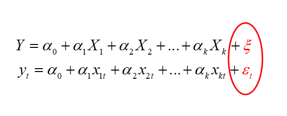
Finally, it is worth noting that “random component” is not the only term used for  (epsilon). You may also encounter other terms such as random disturbance, random error, stochastic component, disturbance, or innovation.
In econometric model notation, the symbol (epsilon) may also be written differently, for example as  (xi),
(xi),  (eta), etc.
As you can see, quite a lot is “contained” within the random component. That is why it is very important to include it every time in the general form of an econometric model — especially since its properties play a crucial role in model verification.
END
Click to review what an econometric model is (previous Lecture) <–
Click to see where statistical data for an econometric model come from (next Lecture) ->
Click to return to the Econometrics Lectures page