Indefinite Integrals Lecture 2
Topic: Indefinite integrals and areas of regions.
Summary
In this lecture I will show a strange (so it would seem) thing. It will turn out that an antiderivative of the function ![]() can be interpreted geometrically as a certain area function associated with this function – something that seems completely unrelated to those velocities and sleds that I drew in the previous lecture.
can be interpreted geometrically as a certain area function associated with this function – something that seems completely unrelated to those velocities and sleds that I drew in the previous lecture.
What should you already know?
Before you start reading, you should already know what an indefinite integral and an antiderivative are (the previous Lecture).
Let’s begin. What function and what area are we talking about?
An indefinite integral is a family of antiderivatives of a certain function ![]() . Antiderivatives, i.e. functions whose derivative equals
. Antiderivatives, i.e. functions whose derivative equals ![]() . Let’s draw our
. Let’s draw our ![]() :
:
")
Is this function already our antiderivative? Of course not – an antiderivative is a function whose derivative gives the drawn ![]() .
.
Let’s stir things up a bit in this drawing and mark the following area:

This is an area that may not be easy to compute (because it is not a basic geometric figure), but it certainly has some definite value, e.g. 10, or ![]() . For the moment, we are not concerned with what it is.
. For the moment, we are not concerned with what it is.
Assuming that ![]() is a constant and shifting
is a constant and shifting ![]() we will obtain some other area:
we will obtain some other area:

And it is clear that by shifting this ![]() (we agree that
(we agree that ![]() is the boundary, i.e.
is the boundary, i.e.  ) we will obtain different values of the area under the function
 ![]() :
:


The area values will change depending on ![]() , so we can say that all areas constructed as above are values of some AREA FUNCTION depending on x. We denote it as:
, so we can say that all areas constructed as above are values of some AREA FUNCTION depending on x. We denote it as:

In general, on the drawing it can be marked like this:
 z funkcją pola P(x)")
We understand that for different arguments x we obtain different values of the area ![]() .
.
So we have two functions:

and
What is the relationship between them?
Ladies and Gentlemen, it is nothing less than this: one is an antiderivative of the other – or in other words, the second is the derivative of the first (from the previous Lecture we know that derivative and antiderivative are sort of “inverse” concepts).
We will show this next.
The area function P(x) is an antiderivative of f(x) – we prove it
Let’s return to our graph and imagine that we shift x not by 1, nor by 10, nor by ![]() units to the right, but by some (for now) unspecified value
units to the right, but by some (for now) unspecified value ![]() :
:
 powiększonego o deltaP")
After such an increment ![]() , our area
, our area ![]() will also increase by
will also increase by ![]() .
.
Now let’s mark the smallest and the largest value of the function ![]() on the interval
on the interval  as
as ![]() and
and ![]() :
:
")
Each of them determines a rectangle (blue and red, respectively):

These are rectangles with one side equal to the segment of length ![]() and the other side equal to
and the other side equal to ![]() or
or ![]() . It is obvious (look at the figure and ask yourself whether it could be otherwise) that our area
. It is obvious (look at the figure and ask yourself whether it could be otherwise) that our area ![]() is greater than the area of the blue rectangle and smaller than the area of the red rectangle, i.e.:
is greater than the area of the blue rectangle and smaller than the area of the red rectangle, i.e.:
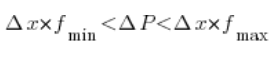
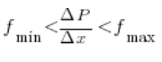
Dividing both sides of these inequalities by ![]() we obtain:
we obtain:
Now an important moment:
If our ![]() tends to
tends to ![]() , i.e. becomes infinitesimally small, then the values
, i.e. becomes infinitesimally small, then the values ![]() and
and ![]() will tend to
will tend to ![]() , i.e. to the value of the function at the point x. Follow this on the last graph and imagine that the increment
, i.e. to the value of the function at the point x. Follow this on the last graph and imagine that the increment ![]() is smaller and smaller and smaller… How will
is smaller and smaller and smaller… How will ![]() and
and ![]() behave? They will get closer and closer to
behave? They will get closer and closer to ![]() (in fact, in our particular drawing already now
(in fact, in our particular drawing already now ![]() ).
).
So if in the inequality:
…for ![]() something happens such that:
something happens such that:
![]() and
and ![]() , it is obvious that
, it is obvious that ![]() (this is stated, for example, by the squeeze theorem).
(this is stated, for example, by the squeeze theorem).
So we have – writing the above symbolically:
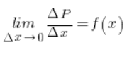
And what is the expression on the left-hand side of the equality? The ratio of the increment of the function value to the increment of the argument for an infinitesimal increment of the argument? As we remember from the lectures on derivatives, this is EXACTLY the derivative of this function.
So we have shown that:

…that is, the derivative of the area function equals the function ![]() , or (which is the same) that:
, or (which is the same) that:
THE AREA FUNCTION ![]() IS AN ANTIDERIVATIVE OF THE FUNCTION
IS AN ANTIDERIVATIVE OF THE FUNCTION ![]()
Formula for the area
So we have the function ![]() and an antiderivative of it, the function
and an antiderivative of it, the function ![]() . The indefinite integral was the family of all antiderivatives of the function. The function
. The indefinite integral was the family of all antiderivatives of the function. The function ![]() is therefore one of these functions. How does it differ from the others? From the previous Lecture we know that antiderivatives differ by a CONSTANT. Therefore, if we take as
is therefore one of these functions. How does it differ from the others? From the previous Lecture we know that antiderivatives differ by a CONSTANT. Therefore, if we take as ![]() any other antiderivative of
any other antiderivative of ![]() , we will get:
, we will get:

If in the equation above we take ![]() , we determine the constant C, i.e. the value by which
, we determine the constant C, i.e. the value by which ![]() differs from any other antiderivative:
differs from any other antiderivative:
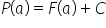
![]() (look at our graph and see what happens when we take
(look at our graph and see what happens when we take ![]() in it), that is:
in it), that is:


So, returning with the determined constant C to the formula ![]() we obtain:
we obtain:
So we have a powerful formula for area. We can compute it… by integrating (finding an antiderivative and substituting appropriate values for ![]() and
and ![]() ). Powerful, because we are no longer limited to areas of circles, triangles, trapezoids (i.e. those for which we have “formulas”). We can calmly compute the area of irregular regions – lakes, forests, or whatever comes to mind.
). Powerful, because we are no longer limited to areas of circles, triangles, trapezoids (i.e. those for which we have “formulas”). We can calmly compute the area of irregular regions – lakes, forests, or whatever comes to mind.
Example
Compute the area between the OX axis and the graph of the function ![]() .
.
On the graph, this area would look like this:

With this (after all very simple) problem, we would be completely helpless knowing only the high-school formulas for a trapezoid, parallelogram, circle, etc. Well, maybe not completely, because we could compute it “approximately” (for example by dividing the area under the parabola into small rectangles). But from today (or rather, since about the 17th century) we have additional artillery.
So we will use our formula for the area function:
We take as our ![]() the “beginning” of the area on the OX axis, i.e.
the “beginning” of the area on the OX axis, i.e. ![]() . We take as x the “end” of the area on the OX axis, i.e.
. We take as x the “end” of the area on the OX axis, i.e. ![]() . An antiderivative (found by integration) of the function
. An antiderivative (found by integration) of the function ![]() is the function
is the function ![]() (a simple integral). So we have:
(a simple integral). So we have:

So the area under the parabola is exactly that. We can prepare the right amount of concrete to pour, or grass seed to plant, or whatever it is we needed 🙂
END
While writing this post, I used:
1. „Differential and Integral Calculus. Vol. II.” G.M. Fichtenholz. 1966 edition.
Click here to remind yourself what an indefinite integral is (previous Lecture) <–
Click here to return to the page with lectures on indefinite integrals