Derivatives of Functions Lecture 1
Topic: An intuitive introduction to the concept of the derivative of a function (the derivative as velocity)
Summary
In this article I will try to explain more clearly what derivatives of functions actually are, starting completely from the basics. To get your teeth into the topic, elementary school math, a calculator, and a good, optimistic attitude at the beginning are enough. I strongly recommend equipping yourself with all three before reading!
Little Johnny on a sled
We’ll start with a concrete example to show you, in general, what’s what with derivatives. Imagine winter, a hill, and a small sledder named Johnny sliding down from the top. We all know the phenomenon that at the beginning the sled moves very slowly, and later it goes faster and faster as it accelerates (assuming an optimal, safe ride for little Johnny). Let’s also imagine that, in order to describe the ride, we measure—very precisely—every second, the distance traveled by the sled. Let’s take distance measurements for the first six seconds of the sled’s motion:

From analyzing the table, we have “in writing” what everyone senses intuitively, namely that the sled does not move uniformly. In the first second of motion little Johnny traveled (can we say that about a sled?) only half a meter, and for example between the measurement at the second and the third second he traveled 2.5 meters in the same time. So at the beginning the sled must have been sliding slowly, and later faster and faster. Derivatives of functions are closely related to velocity.
Let’s plot our measurements on a graph (this is where valuable elementary-school knowledge will come in handy):

Take a moment to connect the graph with the table. You can notice a certain regularity in the dots, right? It was rather hard to see from the bare numbers in the table, which is why graphical representations of various algebraic operations are very important in mathematics. Some people (Descartes) even tried to reduce all of mathematics to geometry! But let’s get back to derivatives.
The dependence of distance on time (by the way, such a dependence is called a function — you’ll still need to wait patiently for derivatives of functions) is not completely random in our model. Look closely at the table. What do the numbers denoting time (0,1,2,3,4,5,6…) have in common with the numbers denoting the distance traveled (0;0,5;2;4,5;8;12,5;18…) that correspond to them?
If you answered correctly that the numbers 0;0,5;2;4,5;8;12,5;18… are halves of the squares of the numbers 0,1,2,3,4,5,6…, then you’re very good at this stuff—congratulations! Look, let’s examine each column in turn:
0 (distance) is equal to half of the square of zero (time) – correct
0,5 (distance) is equal to half of the square of 1 (time), because ![]() – correct
– correct
2 (distance) is equal to half of the square of 2 (time), because ![]() – correct
– correct
4,5 (distance) is equal to half of the square of 3 (time), because ![]() – correct
– correct
8 (distance) is equal to half of the square of 4 (time), because ![]() – correct
– correct
12,5 (distance) is equal to half of the square of 5 (time), because ![]() – correct
– correct
18 (distance) is equal to half of the square of 6 (time), because ![]() – correct.
– correct.
We can say that distance is related to time by the relationship distance=(time^2):2, and if we take distance as s and time as t, in mathematical form: ![]() . To feel more at home, let’s use the letter y for the variable dependent on the other one (distance) and the letter x for the independent variable (time). We then get the formula describing the sled’s motion in the first six seconds:
. To feel more at home, let’s use the letter y for the variable dependent on the other one (distance) and the letter x for the independent variable (time). We then get the formula describing the sled’s motion in the first six seconds:

Such a function can be called a second-degree polynomial. In the days when the concept of the derivative was being created (or when the concept “derivatives of functions” was being discovered — depending on which philosophy of mathematics you accept), polynomials were used to describe many concrete physical phenomena: the pressure of water on dams, the trajectory of an artillery projectile, the motion of stars and planets. The increasing complexity of problems connected with various applications of mathematics created strong pressure to find better and more detailed methods for analyzing functions—simple addition or multiplication was no longer enough. Different scholars, in different ways, by small steps and discoveries, approached the concept of the derivative of a function, which we will also reach in a moment 🙂
And you too—if in your professional career, for example as an engineer or economist, you plan to go beyond—let’s say—the 17th century in the development of human knowledge, you have to go down this road. There are no shortcuts here.
Continuity of a function
Let’s look once again at our table. As a model describing the sled’s motion, it is far from perfect. If it contains no value for time 2.5 seconds, does that mean that at 2.5 seconds of motion the sled covered no distance? That the sled teleported between the second and third second from the second meter to the fourth? Of course not. At 2.5 seconds of motion the sled also covered some distance; we simply did not measure it—just like at 2.99999 seconds of motion, and in general for every time value other than zero the sled covered some distance.
What could that distance be?
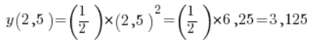
Since we already know that distance is related to time by the relationship ![]() (where y is distance and x is time), we can calculate it easily by squaring 2.5 and dividing the result by 2. Mathematically, we can write:
(where y is distance and x is time), we can calculate it easily by squaring 2.5 and dividing the result by 2. Mathematically, we can write:
If we marked this value on our graph, we would get:

It’s clear that we could also calculate the appropriate distance value at 0.0001 seconds of motion, and in general at any time. For each of them we could plot the corresponding dot. And all those dots would connect into an elegant graph:

Functions of this type, in which for every number x from some interval (in our case from 0 to 6), also for x’s that are fractions or irrational numbers (e.g. ![]() ), there exists a value y, we can call continuous functions. Continuous functions on graphs form nice lines that you can draw without lifting your pen from the paper. Time is a classic example of a continuous quantity. We can talk about 1.9999999 seconds of motion, or about
), there exists a value y, we can call continuous functions. Continuous functions on graphs form nice lines that you can draw without lifting your pen from the paper. Time is a classic example of a continuous quantity. We can talk about 1.9999999 seconds of motion, or about ![]() seconds of motion. One may also assume that height is a continuous value—there is no problem for a person to be 176.000002 cm tall. In contrast—for example—the number of children in a family is not a continuous quantity, because you cannot have 2.49837 children. We arrive here at an important thing:
seconds of motion. One may also assume that height is a continuous value—there is no problem for a person to be 176.000002 cm tall. In contrast—for example—the number of children in a family is not a continuous quantity, because you cannot have 2.49837 children. We arrive here at an important thing:
Derivatives apply only to continuous functions.
The concept of the rate of change
So we have a function describing how the distance traveled by little Johnny changes with time, and we have drawn its graph. Let’s return to the phenomenon we’ve been talking about from the very beginning—namely velocity. At first, for equal changes in time, the distance traveled by the sled increased slowly. After a few seconds, for the same changes in time, that distance increased by larger and larger amounts. Look at the graph—you can see it clearly there. That is velocity, right? It is a measure of the change in distance with respect to time.
How can we measure the sled’s velocity at any moment of its motion in such a described ride? We don’t have a speedometer, remember (we are in the 17th century). Do you have any ideas at this stage?
How to measure velocity? Average velocity
A nice idea for measuring the magnitude of the change in distance with respect to time is simply to divide one by the other. If we travel a distance—say 400 km (let’s leave the sled for a moment)—in 5 hours, then the result is the number of kilometers traveled per 1 hour; that is, 400 divided by 5 gives 80. This means we traveled the whole way at an average of ![]() .
.
Of course, this measure (average velocity) does not convey information about how fast we were going on the highway, whether we took breaks, or how fast we crawled in traffic jams passing through big cities. So it is not yet what we want.
Returning to our sled example for derivatives:
In 6 seconds little Johnny traveled 18 meters (we can read this from the table). This gives the average velocity of his motion: 18:6=3 meters per second. But how do we calculate at what speed Johnny was moving at the 2-second mark of the ride? It certainly was not 3 meters per second… Does such a question even make sense? From life we know it does—but how do we compute it, knowing only the concept of average velocity? What distance increment and what time change should we take, and what should we divide by what? Grab a calculator and compute a bit with me…
We want to calculate the sled’s velocity at 2 seconds of motion.
Let’s first calculate the average velocity (we already know how) of the sled between the 2nd and 3rd second of motion.
The distance traveled between the 2nd and 3rd second is: 4.5 (distance traveled at 3 seconds) – 2 (distance traveled at 2 seconds) = 2.5. Pause here for a moment. This must be completely clear to you.
The time between the 2nd and 3rd second is of course 1 second. Dividing one by the other we get: 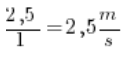 .
.
So between the 2nd and 3rd second the sled was racing at ![]() .
.
Now let’s calculate the average velocity of the sled between 2 and 2.5 seconds of motion.
What distance did the sled cover at 2.5 seconds of motion? We calculated it earlier; we’ll calculate it again. Since distance equals time squared divided by two, we just square 2.5 and divide by 2. I encourage you to use a calculator; we get 3.125.
The distance traveled between 2 and 2.5 seconds will therefore be: 3.125 (distance at 2.5 seconds) – 2 (distance at 2 seconds) = 1.125.
The time between 2 and 2.5 seconds is—attention—0.5 seconds! Dividing one by the other we get (use a calculator): 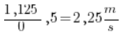 .
.
So between 2 and 2.5 seconds the sled already had a smaller velocity (after thinking about it—this is logical, right?), because ![]() .
.
Which average-velocity calculation seems closer to the exact velocity at 2 seconds of motion: the average velocity between 2 and 3 seconds, or between 2 and 2.5 seconds? Of course the second one. Do you see where this is going?
Now let’s take the average velocity of the sled between 2 and 2.25 seconds of motion.
What distance did the sled cover at 2.25 seconds of motion? We square 2.25 and divide by 2 (calculator). We get 2.53125.
The distance traveled between 2 and 2.25 seconds will therefore be: 2.53125 (distance at 2.5 seconds) – 2 (distance at 2 seconds) = 0.53125.
The time between 2 and 2.25 seconds is 0.25 seconds. Dividing one by the other we get (use a calculator): 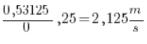 .
.
Now the average velocity of the sled between 2 and 2.1 seconds of motion.
Distance at 2.1 seconds of motion = 2.205.
Distance between 2 and 2.1 seconds = 2.205 – 2 = 0.205.
The time between 2 and 2.1 seconds is 0.1 seconds. Dividing one by the other: 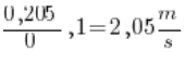 .
.
Computing analogously the velocities between 2 and 2.05 seconds we get the result: ![]()
Between 2 and 2.01 seconds: ![]() .
.
Between 2 and 2.001 seconds: ![]()
So we have successive approximate average velocities, each of which is closer and closer to the exact velocity at 2 seconds of motion:
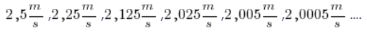
Of course, you don’t need Einstein to notice that these values are getting closer and closer to ![]() . Engineers and scholars in the 16th–17th centuries used this kind of approximation method until they obtained a sufficiently good approximation—so that the dam would not break, the building would not collapse, and the ship would reach its destination.
. Engineers and scholars in the 16th–17th centuries used this kind of approximation method until they obtained a sufficiently good approximation—so that the dam would not break, the building would not collapse, and the ship would reach its destination.
Derivatives of functions at a point
So by taking successive approximations as above, we obtain an increasingly accurate measurement of velocity. When we have obtained a good enough approximation, we can stop the process. Now let’s try to formalize a bit what we did above. We studied the velocity at the second second of motion. Let’s denote ![]() . First we calculated the appropriate segments of distance traveled over successive time intervals; for example, we subtracted the distance at the second second from the distance at the third second. Notice that if we denote the time increments (first 1 second, then half a second, then 0.25 seconds, etc.) as
. First we calculated the appropriate segments of distance traveled over successive time intervals; for example, we subtracted the distance at the second second from the distance at the third second. Notice that if we denote the time increments (first 1 second, then half a second, then 0.25 seconds, etc.) as ![]() , then the corresponding distance increments can be denoted as:
, then the corresponding distance increments can be denoted as: ![]() , where
, where  denotes the distance traveled at 3; 2.5; 2.25 seconds and so on, and
 ![]() — the distance at the second second.
— the distance at the second second.
We computed successive average velocities using the formula:
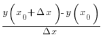
Later we took smaller and smaller values of ![]() . Intuitively we sensed that the values obtained in this way “tend” to 2—without formally stating what that “tend” means precisely. It may be hard to believe, but such intuitive use of calculations involving infinities (specifically infinitely small values) was completely sufficient for many, many years. A formal and rigorous definition of derivatives still had to wait many years. This operation—checking what an expression “tends to”—can be written as:
. Intuitively we sensed that the values obtained in this way “tend” to 2—without formally stating what that “tend” means precisely. It may be hard to believe, but such intuitive use of calculations involving infinities (specifically infinitely small values) was completely sufficient for many, many years. A formal and rigorous definition of derivatives still had to wait many years. This operation—checking what an expression “tends to”—can be written as:
– that is, as the limit (“limes”) that the expression “approaches” as ![]() “approaches” zero.
“approaches” zero.
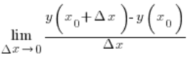
The time has come for the long-awaited derivatives of functions. The derivative of a function at the point ![]() can be described precisely by such a limit:
can be described precisely by such a limit:
Does this mean that mechanical velocity at some moment (e.g. the motion of a sled, a car, a bicycle, a block on an inclined plane) is exactly the derivative of a function at a point? Exactly so. But this concept is much broader and does not have to be limited to analyzing mechanical motion.
Derivatives of functions in applications
In the formula for the derivative of a function at a point, we divide the increment of the function’s values (the y’s) by the increment of the function’s arguments (the x’s). So as a result we obtain how many times the increment of the function’s value is larger than the increment of the argument. In other words, we obtain a measure of “how fast” the graph of any function grows—not necessarily one describing the motion of physical objects. It could be an increase in temperature, pressure, consumer optimism index, or stock market prices! The possibilities are endless, because just imagine—everything that changes can change at different speeds. And if we want to study that speed in a strict way, not just “more or less,” we must use derivatives.
Often it is the other way around—we know the rate of change, but we do not know the function that describes the changes—then we have to use the operation inverse to taking a derivative—namely an integral.
Derivatives of functions as other functions
In the sled example we studied the derivative at a specific point {{x}_{0}}=2 and obtained the specific value 2. It is not hard to imagine that we could similarly study derivatives of the function at any other point {{x}_{0}}=1, {{x}_{0}}=0,5, or {{x}_{0}}=4. The obtained derivative values would also not be completely chaotic (I even invite you to compute them yourself), but they would form a function ![]() , i.e. the derivative at the point {{x}_{0}}=1 would come out equal to 1, and so on.
, i.e. the derivative at the point {{x}_{0}}=1 would come out equal to 1, and so on.
What does this mean? If we get a derivative at some point equal to 10, we know that at that point the increment of the function’s value is 10 times greater than the increment of the argument—the graph rises very steeply upward, and the phenomenon described by the function changes quickly. If the derivative comes out equal to, for example, ![]() , the change does not happen very quickly.
, the change does not happen very quickly.
The derivative of a function at any point, not just at some specific one, is computed from the formula (by definition):
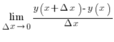
As a result we will of course obtain another function. To make calculations easier, we can also use formulas and properties of derivatives.
THE END
Click to see another way to understand derivatives of functions (next Lecture) –>