How to Understand What Multivariable Functions Are

Understanding from the very basics what a function of two or three variables actually is is extremely important for you. Why, if this is just one of many topics in mathematical analysis?

Because a huge number of things are based on multivariable functions: partial derivatives, multiple integrals, half of physics, three quarters of mechanics, and quite a lot of economics.

Functions of one variable – a reminder

Before higher education, you were introduced to the concept of a function of one variable. A function depending on a single argument.

Such functions could be, for example:

f\left( x \right)={{x}^{2}} – the function assigns to arguments x the values of those arguments squared. That is, to the number 1 it assigns the number 1, to the number 2 the number 4, to the number -3 the number 9, etc.

y=x – the function assigns to arguments x values equal simply to those arguments. That is, to the number 1 it assigns the number 1, to the number 2 the number 2, to the number -3 the number -3, etc.

If we agree that the radius of a circle is the argument r, then the area of a circle is also a function of one variable (it depends only on r) P=\pi {{r}^{2}}. It assigns to radius 1 an area of approximately 3.14, to radius 2 an area of about 12.56, etc.

Functions of one variable can also be:

• distance as a function of time (argument = time, value = distance)
• revenue as a function of the number of customers entering a store (argument = number of customers, value = revenue)
• an exam grade as a function of the percentage of points obtained (argument = percentage, value = grade)
• the number of seats in parliament as a function of the number of votes cast (argument = number of votes, value = number of seats)
• income as a function of education level (argument = education, value = income)

When it comes to numerical functions (assigning numbers to numbers), you have already learned a neat way to “visualize” them, namely a 2-dimensional graph with X and Y axes.

Functions of two variables

Functions of two variables – introduction, examples

If you think about it for a moment, the concept of a function of one variable practically begs to be extended. After all, there are plenty of things around us that change depending on two factors, not just one.

For example, even the simple volume of a cylinder from middle school depends on:

• the radius of its base
• its height

…and is described by the formula: V=\pi {{r}^{2}}H

The values of V change depending on both arguments r and H. Moreover, one can notice that the same increases in r and H do not cause equal increases in V. The volume is more “sensitive” to changes in the base radius – increasing the radius causes the volume to increase faster than increasing the height (at least in most cases).

Other examples include:

• electrical resistance R=\frac{U}{I} depending on voltage and current (argument 1 = voltage, argument 2 = current, value = resistance)
• company revenue depending on price and quantity of goods sold (argument 1 = price, argument 2 = quantity, value = revenue)
• the speed of a balloon flight depending on wind strength and direction (argument 1 = strength, argument 2 = direction, value = speed)
• the size of a purchased hamburger depending on the amount of money in your pocket and the level of hunger (argument 1 = money, argument 2 = hunger, value = size)
• the amount of car insurance premium depending on age and the number of collisions in the past year (argument 1 = age, argument 2 = number of collisions, value = premium)

Of course, the way such functions are plotted on a graph must change.

Pairs of arguments can be plotted on the XY plane, and an additional axis – the Z axis – is used for the values. Therefore, the graph must necessarily be three-dimensional.

Watch this video in which I show how such a graph is created:

https://www.youtube-nocookie.com/embed/_u4VP1U4Fbs?si=AOLn6yOBI2QOnm7D

I am also including a few other graphs of functions of two variables:

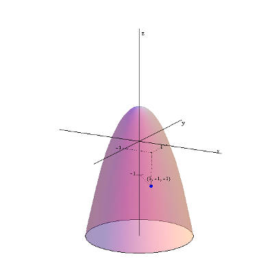
f\left( x,y \right)=1-{{x}^{2}}-{{y}^{2}} with the value marked at the point (1,-1):

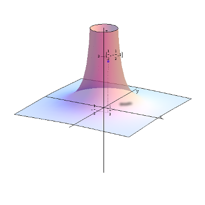
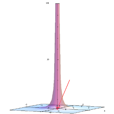
f\left( x,y \right)=\frac{1}{{{x}^{2}}+{{y}^{2}}} with the value marked at the point \left( \frac{1}{2},-\frac{1}{2} \right):

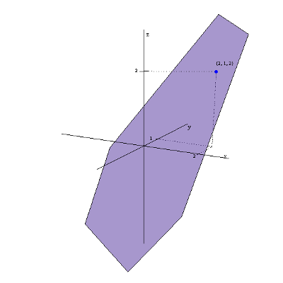
f\left( x,y \right)=x+y-1 with the value marked at the point \left( 2,1 \right):

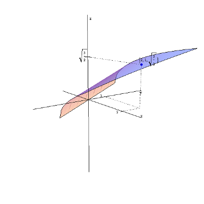
f\left( x,y \right)=\sqrt{x+\frac{y}{2}} with the value marked at the point \left( 2,1 \right):

Domain (range of variability of arguments) of functions of two variables

Theory

In the case of a function of one variable f\left( x \right), the domain of the function was the set of arguments x that can be substituted into it at all in order to obtain some value.

For example, for the function f\left( x \right)=\frac{1}{x} , you could substitute any value of x except 0 (because that would be division by zero), so its domain was the set of all real numbers except 0 ( R\backslash \left\{ 0 \right\}).

In the case of a function of two variables f\left( x,y \right), the domain of the function will still be those arguments x and y that can be substituted into it.

For example, for the function f\left( x,y \right)=\frac{1}{x+y} , you can substitute any values of x and y except those for which y=-x (because that would result in division by zero), so its domain is the set of all pairs of real numbers (x,y) such that y\ne -x.

This domain could be represented on the plane by shading the entire plane EXCEPT the line y=-x.

Practice

In practice, you determine the domain of a function of two variables using the same “restrictions” as for a function of one variable, namely:

• you cannot divide by zero
• you can only take the square root of a non-negative number
• you can only take the logarithm of a positive number

Example 1

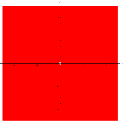
Find the domain of the function f\left( x,y \right)=\frac{1}{{{x}^{2}}+{{y}^{2}}}.

In the formula for the function, you have division. You know that in such a case the denominator must be non-zero, so the restriction takes the form:

{{x}^{2}}+{{y}^{2}}\ne 0

{{x}^{2}}+{{y}^{2}} is equal to zero if and only if x and y are BOTH equal to zero.

The domain of this function therefore consists of all values of x and all values of y, except x=0 and y=0 simultaneously.

Example 2

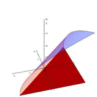
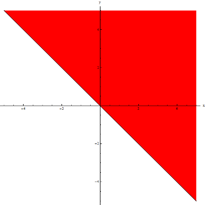
Find the domain of the function f\left( x,y \right)=\sqrt{x+y}.

In the formula for the function, you have a square root. You know that the argument of the square root must be greater than or equal to 0.

Therefore:

x+y\ge 0

That is:

y\ge -x

The domain of this function is the set of all points on the plane with coordinates such that y\ge -x.

The most convenient way to represent this is geometrically, as points lying on and above the line y=-x:

Example 3

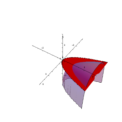
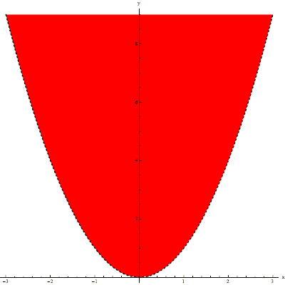
Find the domain of the function f\left( x,y \right)=\ln \left( y-{{x}^{2}} \right).

The argument of a logarithm can only be a positive number, therefore:

y-{{x}^{2}}>0

That is:

y>{{x}^{2}}

The domain of the function is therefore the set of all points whose y-coordinates are greater than the x-coordinates squared. Graphically, this will be the area ABOVE the parabola y={{x}^{2}}, but WITHOUT the parabola itself:

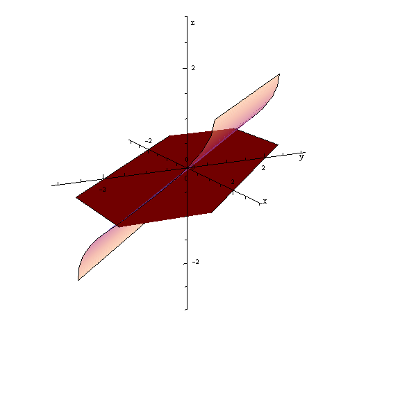
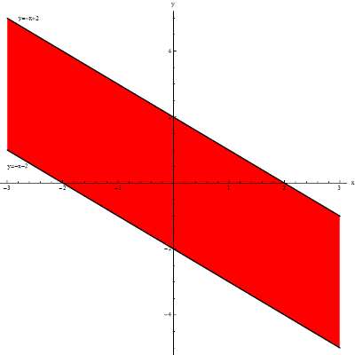
Example 4

Find the domain of the function z=\arcsin \frac{x+y}{2}.

Arcus sine is a somewhat less commonly used function. The restriction on its domain is that its argument must belong to the interval \left\langle -1,1 \right\rangle , therefore:

\frac{x+y}{2}\ge -1\quad \wedge \quad \frac{x+y}{2}\le 1 x+y\ge -2\quad \wedge \quad x+y\le 2 y\ge -x-2\quad \wedge \quad y\le -x+2

The domain of the function consists of all points satisfying both of these conditions simultaneously. Geometrically, this is the area between these two lines, including the lines themselves:

More video examples

I solve and explain more examples (also more difficult ones) step by step in video form in my Multivariable Functions Course. Lesson 5 of the course is dedicated specifically to finding the domain of functions of two variables. I also discuss the general scheme for determining domains in more detail there. You’re welcome if you want to explore this topic further and learn how to find domains with more than one restriction (e.g. division and square root in a single function).

Homework

If you want to test yourself a bit, here is a small homework assignment.

Find the domain of the following functions:

1. f\left( x,y \right)=\frac{1}{x+y+3}
2. f\left( x,y \right)=\frac{1}{x-2y}+15xy
3. z=\sqrt{x-y}
4. z=\ln \left( y-2+3x-{{x}^{2}} \right)

Functions of three and more variables

Since functions of one variable can be extended to functions of two variables, there is really no logical reason to stop there.

It is easy to imagine functions of three ( f\left( x,y,z \right)), four ( f\left( x,y,z,u \right)), or even any number of variables (

f\left( {{x}<em>{1}},{{x}</em>{2}},\ldots ,{{x}_{n}} \right)

).

From a mathematical point of view, there is no problem analyzing such functions using the same principles as for functions of one variable. That means computing their limits, derivatives, extrema, and domains.

In practice, however, a certain barrier appears, related more to human perception of the world than to mathematics. The issue is graphs.

Let us consider a function of three variables f\left( x,y,z \right)={{x}^{2}}+{{y}^{2}}+{{z}^{2}}. Its domain is the set of triples (x,y,z), which we can represent on a three-dimensional graph. The point (1,1,2) clearly belongs to this domain, because it can be substituted into the function (thus obtaining its value: {{1}^{2}}+{{1}^{2}}+{{2}^{2}}=6).

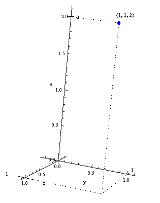
The question is: where should we mark the value of the function, i.e. 6?

The ‘z’ axis in this graph is used to represent the third argument, not the value (as was the case for graphs of functions of two variables).

To somehow represent this value geometrically, we would have to, as it is often said colloquially, “enter the fourth dimension”, which for obvious reasons is very difficult. One possible idea is to use color coding (e.g. the colder/bluer the color, the smaller the value; the warmer/redder, the larger the value), but the limitations of such methods are fairly obvious.

For functions of four variables, we already give up on drawing graphs at the domain stage.

The fact that we cannot draw or even visualize something in our minds does not mean that we cannot compute it. That is why I want to emphasize once again that the only real problem with functions of more than two variables is their geometric representation.

Next lecture

You now know what multivariable functions are and how they can be “imagined”. You also know when they cannot be imagined 🙂

We therefore move on to further analysis. Do you remember from functions of one variable what came after finding the domain and getting familiar with the graph? Yes, exactly. Limits.

While writing this post, I used…

1. “Differential and Integral Calculus. Volume I.” G.M. Fichtenholz. Edition 1966.