
Econometrics Lecture 2
Topic: Econometric Model
In the previous Lecture 1, I tried to explain what econometrics is and what it deals with.
Like any economic or mathematical discipline, econometrics has its basic tools used to study quantitative relationships. This practical tool is precisely the econometric model.
In this article, I will try to break this concept down into its basic components.
So let’s get started.
The concept of an econometric model
As I mentioned at the beginning, the basic tool used in econometric analysis is the econometric model.
A “model” is a formal theoretical construct that is analyzed instead of the real phenomenon itself. It is a kind of simplified representation of reality. By “simplified”, I mean including only the most important elements of reality in the model and omitting the less significant ones. You will probably agree with me here — we are simply not able to take into account absolutely all possible factors.
Example 1
Mr. Janusz has been running a used car dealership for several years. He decided to explain what determines the sales value of the cars offered there. After carefully analyzing all possibilities, he came to conclusions that surprised even him. He never would have thought that car sales depend on so many factors: price (obviously), but also the brand of the car, its age, mileage, technical condition, whether it has been in an accident, country of origin, color, number of previous owners, number of advertisements in newspapers, number of online advertisements, number of accidents in the city, season of sale, advertising expenses of the dealership, number of rainy days, number of snowy and frosty days…
He could go on listing them almost endlessly.
If Mr. Janusz wanted to build a model explaining sales, would he really have to take all these data into account? Of course, that would not be entirely reasonable.
As you can probably see, some variables have a strong and lasting impact. Others are weaker and short-lived. In addition, one must account for the influence of so-called random factors — sudden, irregular events that nevertheless have a significant impact (for example, the theft of several cars from the dealership).
Returning to the concept of the econometric model, a very precise definition was formulated by the Polish econometrician Zbigniew Pawłowski:
“An econometric model is a formal construct which, by means of a single equation or a system of equations, represents the essential relationships occurring between the analyzed economic phenomena.”
Thus, it is an equation — a certain mathematical representation that has been “fitted” to reality using appropriate statistical methods. Importantly, only the most essential variables are included.
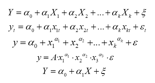
This is the most general form of the model:

What does it consist of? It has several constant elements:
a) First, the variable you want to explain using the model. It is called the dependent variable. It is most often denoted by “” and appears on the left-hand side of the equation. It is also often called the “dependent variable” because it depends on other variables that influence it.
In our example,  could represent the “sales value of cars”.
b) The next element is the variable or variables used to EXPLAIN the behavior of the dependent variable. This is where your own knowledge, a bit of experience, and some imagination come in handy — just like in Mr. Janusz’s case, where he identified several such variables. They are most often denoted as:  . These are the explanatory variables, located on the right-hand side of the equation. They are also called “independent variables”, since they do not depend on other variables and have their own economic meaning.
c) In the equation, you can see a peculiar symbol  , resembling a handwritten “E”. This is epsilon, a Greek letter. It denotes a random variable — the so-called random error term or disturbance.
A mathematical equation is always treated as an approximation. Therefore, the random component accounts for, among other things: differences between the model and reality, the influence of omitted variables, measurement errors, and unexpected random factors.
I recommend reading more about this in the next Lecture — you will see that it is a very important part of the model.
d) The function  represents the type of functional relationship between the dependent variable, the explanatory variables, and the random component.
This concerns how the variables are “connected” — whether linearly (added together), multiplied, or perhaps expressed using logarithms. The function  describing the relationships between explanatory variables can take any form (exponential, logarithmic, rational, or a combination of several). The choice here is unlimited.
e) As you can see in the examples above, besides  and
and  , there are other symbols as well — here denoted as
  . These are scalars — numerical values by which variables are multiplied. They are called structural parameters. Of course, you could use any symbols you like, even simple ones such as
  . However, in general econometric model notation, Greek letters (alpha, beta, gamma, etc.) are used most often.
If we wanted to build a simple econometric model for Mr. Janusz (from Example 1), it could look like this:

I assumed a linear relationship between variables (to simplify later calculations).
I deliberately did not include all the characteristics mentioned by Mr. Janusz — it would not make sense. Such a model would simply be too extensive. Moreover, including too many variables is not always advisable. The theoretical values of the dependent variable , calculated based on the model, would likely be too far from the actual sales results. The model would simply not be “well fitted” to the economic variables.
I will explain what this “fitting” of the model to data means in the following Lectures.
I will also mention (this might come in handy for an exam) that econometricians distinguish two types of econometric models depending on whether the so-called “random component” is included or not. This is why it is such an important element.
STOCHASTIC MODELS – models that include a random component, that is . These models occur in about  of cases.
DETERMINISTIC MODELS – models that do not include a random component, that is  . This is simply a concrete function, for example the well-known straight line
  .
.
Where does this difference come from? The random component includes, among other things, omitted variables as well as measurement and calculation errors. This property makes the model closer to real-world phenomena — what actually happens in reality. After all, we are never able to determine perfectly exact functional relationships.
Therefore, it should be remembered that inference based on a stochastic model, after estimating its parameters, is only approximate in nature.
Now that we know what our model looks like, all that remains is to collect appropriate data, specify the model, estimate it (that is, compute numerical values of the structural parameters), verify it, and apply it — the subsequent stages of econometric modeling.
I encourage you to read my subsequent Lectures and to familiarize yourself with my Course.
END
Click to review what econometrics is (previous Lecture) <–
Click to learn about the role of the random component in an econometric model (next Lecture) ->
Click to return to the Econometrics Lectures page